Client-side (local) processing#
Warning
This is a new experimental feature and API, subject to change.
Background#
The client-side processing functionality allows to test and use openEO with its processes locally, i.e. without any connection to an openEO back-end. It relies on the projects openeo-pg-parser-networkx, which provides an openEO process graph parsing tool, and openeo-processes-dask, which provides an Xarray and Dask implementation of most openEO processes.
Installation#
Note
This feature requires Python>=3.9.
Tested with openeo-pg-parser-networkx==2023.5.1 and
openeo-processes-dask==2023.7.1.
pip install openeo[localprocessing]
Usage#
Every openEO process graph relies on data which is typically provided by a cloud infrastructure (the openEO back-end). The client-side processing adds the possibility to read and use local netCDFs, geoTIFFs, ZARR files, and remote STAC Collections or Items for your experiments.
STAC Collections and Items#
Warning
The provided examples using STAC rely on third party STAC Catalogs, we can’t guarantee that the urls will remain valid.
With the load_stac process it’s possible to load and use data provided by remote or local STAC Collections or Items.
The following code snippet loads Sentinel-2 L2A data from a public STAC Catalog, using specific spatial and temporal extent, band name and also properties for cloud coverage.
>>> from openeo.local import LocalConnection
>>> local_conn = LocalConnection("./")

>>> url = "https://earth-search.aws.element84.com/v1/collections/sentinel-2-l2a"
>>> spatial_extent = {"west": 11, "east": 12, "south": 46, "north": 47}
>>> temporal_extent = ["2019-01-01", "2019-06-15"]
>>> bands = ["red"]
>>> properties = {"eo:cloud_cover": dict(lt=50)}
>>> s2_cube = local_conn.load_stac(
...     url=url,
...     spatial_extent=spatial_extent,
...     temporal_extent=temporal_extent,
...     bands=bands,
...     properties=properties,
... )
>>> s2_cube.execute()
<xarray.DataArray 'stackstac-08730b1b5458a4ed34edeee60ac79254' (time: 177,
                                                                band: 1,
                                                                y: 11354,
                                                                x: 8025)>
dask.array<getitem, shape=(177, 1, 11354, 8025), dtype=float64, chunksize=(1, 1, 1024, 1024), chunktype=numpy.ndarray>
Coordinates: (12/53)
  * time                                     (time) datetime64[ns] 2019-01-02...
    id                                       (time) <U24 'S2B_32TPR_20190102_...
  * band                                     (band) <U3 'red'
  * x                                        (x) float64 6.52e+05 ... 7.323e+05
  * y                                        (y) float64 5.21e+06 ... 5.096e+06
    s2:product_uri                           (time) <U65 'S2B_MSIL2A_20190102...
    ...                                       ...
    raster:bands                             object {'nodata': 0, 'data_type'...
    gsd                                      int32 10
    common_name                              <U3 'red'
    center_wavelength                        float64 0.665
    full_width_half_max                      float64 0.038
    epsg                                     int32 32632
Attributes:
    spec:        RasterSpec(epsg=32632, bounds=(600000.0, 4990200.0, 809760.0...
    crs:         epsg:32632
    transform:   | 10.00, 0.00, 600000.00|\n| 0.00,-10.00, 5300040.00|\n| 0.0...
    resolution:  10.0
Local Collections#
If you want to use our sample data, please clone this repository:
git clone https://github.com/Open-EO/openeo-localprocessing-data.git
With some sample data we can now check the STAC metadata for the local files by doing:
from openeo.local import LocalConnection

local_data_folders = [
    "./openeo-localprocessing-data/sample_netcdf",
    "./openeo-localprocessing-data/sample_geotiff",
]
local_conn = LocalConnection(local_data_folders)
local_conn.list_collections()
This code will parse the metadata content of each netCDF, geoTIFF or ZARR file in the provided folders and return a JSON object containing the STAC representation of the metadata. If this code is run in a Jupyter Notebook, the metadata will be rendered nicely.
Tip
The code expects local files to have a similar structure to the sample files provided at github.com/Open-EO/openeo-localprocessing-data. If the code can not handle you special netCDF, you can still modify the function that reads the metadata from it (openeo/local/collections.py#L19) and the function that reads the data (openeo/local/processing.py#L26).
Local Processing#
Let’s start with the provided sample netCDF of Sentinel-2 data:
>>> local_collection = "openeo-localprocessing-data/sample_netcdf/S2_L2A_sample.nc"
>>> s2_datacube = local_conn.load_collection(local_collection)
>>> # Check if the data is loaded correctly
>>> s2_datacube.execute()
<xarray.DataArray (bands: 5, t: 12, y: 705, x: 935)>
dask.array<stack, shape=(5, 12, 705, 935), dtype=float32, chunksize=(1, 12, 705, 935), chunktype=numpy.ndarray>
Coordinates:
  * t        (t) datetime64[ns] 2022-06-02 2022-06-05 ... 2022-06-27 2022-06-30
  * x        (x) float64 6.75e+05 6.75e+05 6.75e+05 ... 6.843e+05 6.843e+05
  * y        (y) float64 5.155e+06 5.155e+06 5.155e+06 ... 5.148e+06 5.148e+06
    crs      |S1 ...
  * bands    (bands) object 'B04' 'B03' 'B02' 'B08' 'SCL'
Attributes:
    Conventions:  CF-1.9
    institution:  openEO platform - Geotrellis backend: 0.9.5a1
    description:
    title:
As you can see in the previous example, we are using a call to execute() which will execute locally the generated openEO process graph. In this case, the process graph consist only in a single load_collection, which performs lazy loading of the data. With this first step you can check if the data is being read correctly by openEO.
Looking at the metadata of this netCDF sample, we can see that it contains the bands B04, B03, B02, B08 and SCL. Additionally, we also see that it is composed by more than one element in time and that it covers the month of June 2022.
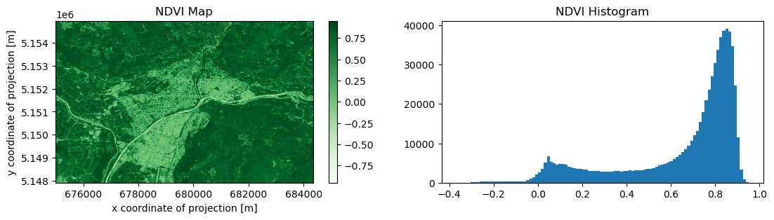
We can now do a simple processing for demo purposes, let’s compute the median NDVI in time and visualize the result:
b04 = s2_datacube.band("B04")
b08 = s2_datacube.band("B08")
ndvi = (b08 - b04) / (b08 + b04)
ndvi_median = ndvi.reduce_dimension(dimension="t", reducer="median")
result_ndvi = ndvi_median.execute()
result_ndvi.plot.imshow(cmap="Greens")
We can perform the same example using data provided by STAC Collection:
from openeo.local import LocalConnection

local_conn = LocalConnection("./")

url = "https://earth-search.aws.element84.com/v1/collections/sentinel-2-l2a"
spatial_extent = {"east": 11.40, "north": 46.52, "south": 46.46, "west": 11.25}
temporal_extent = ["2022-06-01", "2022-06-30"]
bands = ["red", "nir"]
properties = {"eo:cloud_cover": dict(lt=80)}
s2_datacube = local_conn.load_stac(
    url=url,
    spatial_extent=spatial_extent,
    temporal_extent=temporal_extent,
    bands=bands,
    properties=properties,
)

b04 = s2_datacube.band("red")
b08 = s2_datacube.band("nir")
ndvi = (b08 - b04) / (b08 + b04)
ndvi_median = ndvi.reduce_dimension(dimension="time", reducer="median")
result_ndvi = ndvi_median.execute()